Adversarial Attacks

22 June 2021 - 18 mins read time
Tags: Neural network Attack

With recent technological advances, the use of deep neural networks (DNN) have widespread to numerous applications ranging from biomedical imaging to the design of autonomous vehicle. The reasons of their prosperity strongly rely on the increasingly large datasets becoming available, their high expressiveness and their empirical successes in various tasks (e.g. computer vision, natural language processing or speech recognition).

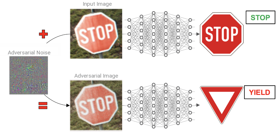
However, their high representation power is also a weakness that some adversary might exploit to craft adversarial attacks which could potentially lead the DNN model to take unwanted actions. More precisely, adversarial attacks are almost imperceptible transformations aiming to modify an example well classified by a DNN into a new example, called adversarial, which is itself wrongly classified. From a fast one-shot method [Goodfellow et al., 2015] to the first iterative procedures [Moosavi-Dezfooli et al., 2016] [Kurakin et al., 2017] [Carlini and Wagner, 2017] , the crafting of adversarial perturbations has lately received a lot of attention from the machine learning community. In this post, I try to review some of the latest developments.

1. Quick reminder about classification based DNN

Before introducing adversarial attacks, we report a quick reminder about classification based deep neural networks.

Let some dataset $\mathcal{D}=\{x_i,y_i\}_{i=1}^n$ made of $n$ samples $x_i\in\mathcal{X}\subseteq\mathbb{R}^P$ and $y_i\in\mathbb{R}^c$. In addition, let some neural network $f\colon\mathcal{X}\to \mathbb{R}^c$ mapping each input $x\in\mathcal{X}$ to its probabilities $f(x)\in\mathbb{R}^c$ to belong to each of the $c$ classes. Then, the usual way to train $f$ on $\mathcal{D}$ consists in solving

\[\underset{f}{\text{minimize}} \sum_{i=1}^n H(f(x_i),y_i)\]

where $H$ is some similarity measure typically chosen as the cross-entropy. There, the minimization over $f$ is intended over the parameters (weights and biases) of the neural network $f$.

Once $f$ is properly trained, the predicted label of any input $x\in\mathcal{X}$ by $f$ is denoted as

\[C_f(x) = \underset{i\in\{1,\ldots,c\}}{\mathrm{argmax}}\, f_i(x).\]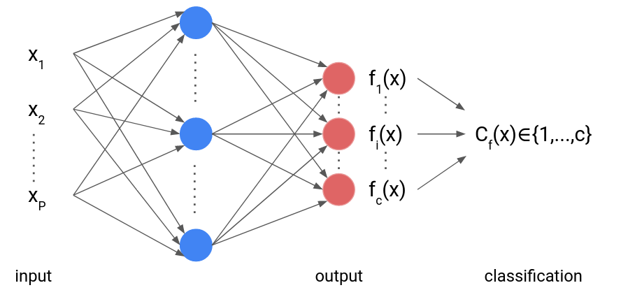

Classification based DNN

2. Span of adversarial attacks

Although DNN have shown a great success to predict various complex tasks, some concerns have been raised about their safety and more particularly for the safety of the user since the pioneer work of [Szegedy et al., 2014] which has shown the existence of adversarial attacks. The most striking example is probably that of automated vehicles where malicious attacks could lead the car to take unwanted action with dramatic consequences.

Adversarial attack

There exist multiple definition of adversarial examples depending on whether we enforce that the adversarial example yields a specific target predicted by the DNN $f$ or not.

Untargeted and targeted attacks. Given some valid input instance $x\in\mathcal{X}$, the adversarial example $a$ is said to be

Untargeted if $C_f(a)\neq C_f(x)$.
Targeted, with target $t\neq C_f(x)$, if $C_f(a)=t$.

In addition, there exist two main ways of crafting such adversarial example.

Perturbation and functional attacks. Given some valid input instance $x\in\mathcal{X}$, the adversarial example $a$ is said to be

Pertubation-based if $a=x+\varepsilon$ for some perturbation $\varepsilon$ small enough.
Functional-based if $a=h(x)$ where $h$ models a small degradation operator.

The key question then becomes exactly how much distortion we must add to cause the classification to change. In each domain, the distance metric that we must use is different. In the space of images, many works suggest that $\ell_p$ norms are reasonable approximations of human perceptual distance. It should be noted that most common methods focus on perturbation-based attacks. Henceforth, it what follows we will solely consider those types of attacks. Furthemore, we will distinguish between per-instance and universal perturbations.

Per-instance and universal attacks. Given some data distribution $\mu$ on $\mathcal{X}$, we consider two types of perturbations, namely

Per-instance if for every $x\sim\mu$ there exist $\varepsilon(x)$ such that $a=x+\varepsilon(x)$ is an adversarial example.
Universal if there exist $\varepsilon$ such that for every $x\sim\mu$, $a=x+\varepsilon$ is an adversarial example

Equipped with these definitions, we now report the performance criteria used to evaluate the quality of the attacks.

Performance criteria. Let some set $\{x_i,a_i\}_{i=1}^n$ made of $n$ instances $x_i$ and their adversarial examples $a_i$ crafted by means of some attack strategy on the neural network $f$. In order to judge upon the quality of the attack, the most common criteria are the following.

Fooling rate: the fraction of adversarial examples which do fool the classifier, i.e., $\frac{1}{n} \sum_{i=1}^n \mathbb{1}_{C_f(x_i)\neq C_f(a_i)}$. Note that in some cases where $f$ is not very accurate, some authors prefer to solely consider the instances where $C_f(x_i)$ correctly predicts the true label.
Computational complexity: Cost of the algorithm used to craft adversarial examples.
$\ell_p$-budget: the amount of distortion/perturbation measured in terms of mean $\ell_p$-norm, i.e., $\frac{1}{n}\sum_{i=1}^n \|a_i-x_i\|_p$.
Transferability: the fooling rate obtained on a neural network $f^\prime$ different from $f$.

Every attack will necessarily face a trade-off between some or all these performance criteria. On the one hand, it is fair to say that the computational cost and the transferability of the attack are mostly related to the algorithmic solution devised. On the other hand, the trade-off between fooling rate and $\ell_p$-budget is rather impacted by the choice of the attack model. Actually, this discrimination is over-simplistic. The reality is way more subtle. Indeed, as we will see, finding an adversarial example amounts in solving a non-convex optimization problem. Hence, the choice of the algorithmic solution will also play a significant role on both the achieved fooling rate and the $\ell_p$-budget. Conversely, some models have been devised to specifically improve transferability.

Let us note that the computational complexity of universal attacks is of $\mathcal{O}(1)$ since, once the universal perturbation $\varepsilon$ is found, an adversarial attack $a^\prime$ to an unseen example $x^\prime$ is built simply by adding $\varepsilon$, i.e., $a^\prime=x^\prime+\varepsilon$. While they benefit from low computational cost, their universality usually goes in pair with poor fooling rates.

3. Per-instance attacks

In this section, we present the most common per-instance attacks. In addition, below, we differentiate between two categories. The first aims at finding the smallest $\ell_p$-budgeted perturbation given some trade-off or constraint on its fooling ability. The second assumes a maximal $\ell_p$-budget $\delta>0$ and looks for an adversarial example inside the $\ell_p$ ball of radius $\delta$ centered in $x$.

3.1. Minimum norm and regularization-based perturbations

L-BFGS [Szegedy et al., 2014] $\ell_2$. This work is the first that noticed the existence of adversarial examples for image classification. Given some adversarial target $t\neq C_f(x)$, solve

\[\underset{\varepsilon\in\mathbb{R}^P}{\mathrm{minimize}}\; \lambda \|\varepsilon\|_2 + H(f(x+\varepsilon,t))\quad\text{s.t.}\quad x+\varepsilon\in\mathcal{X}\]

where the regularization parameter $\lambda>0$ is determined by line-search in order to ensure that $C_f(x+\varepsilon)=t$. The authors have considered the case where $\mathcal{X}=[0,1]^P$ so that the constraint enforces the $P$ pixels to lie inside a box. In addition, they have promoted the use of a box-constrained L-BFGS solver, which hence gave its name to such adversarial crafting technique.

DeepFool [Moosavi-Dezfooli et al., 2016] $\ell_2$. A more elaborated, yet similar approach, consists in finding the adversarial perturbation $\varepsilon(x)$ as the solution of the following optimization problem

\[\underset{\varepsilon\in\mathbb{R}^P}{\mathrm{minimize}}\; \|\varepsilon\|_2\quad\text{s.t.}\quad C_f(x+\varepsilon) \neq C_f(x)\]

CW [Carlini and Wagner, 2017] $\ell_2$. A similar idea to DeepFool is pursued by Carlini and Wagner by considering the fooling requirement as a regularization instead of a constraint, i.e.,

\[\underset{\varepsilon\in\mathbb{R}^P}{\mathrm{minimize}}\; \|\varepsilon\|_2 + \lambda g(x+\varepsilon)\]

where the first term penalizes the $\ell_p$-norm of the added perturbation while the second term enforces the fooling of the DNN classifier $f$ by means of the function $g$.

LogBarrier [Finlay et al., 2019] $\ell_p$. Let $k=C_f(x)$ be the predicted target of $x$ by the DNN $f$. If it is well trained then it should correspond to the label $y$. Thus, a necessary and sufficient condition for a misclassified adversarial example $x+\varepsilon$ is to have $\max_{i\neq k} f_i(x+\varepsilon) - f_k(x+\varepsilon)>0$ with $\varepsilon$ small. On the one hand, a small perturbation $\varepsilon$ can be found by minimizing a criterion $\ell$. One the other hand, the misclassication constraint can be enforced through a negative logarithm penalty (i.e., a logarithmic barrier) weighted by a regularization parameter $\lambda>0$. The resulting problem reads

\[\underset{\varepsilon\in\mathbb{R}^P}{\mathrm{minimize}}\; \|\varepsilon\|_p - \lambda \log\left( \max_{i\neq k} f_i(x+\varepsilon) - f_k(x+\varepsilon)\right)\]

3.2. Maximum allowable perturbations

Most of the attacks presented in this section intend to craft the adversarial perturbation $\varepsilon$ by efficiently or approximatively solving the following optimization problem.

$$\underset{\varepsilon\in\mathbb{R}^P}{\text{maximize}}\, H(f(x+\varepsilon),y)$$

The adversarial example is then defined as $a=\mathcal{P}_{\mathcal{X}}(x+\varepsilon)$, i.e., by projecting the perturbed example into the space of admissible instances.

In what follows, we restrict to untargeted attacks. Their targeted counterpart can easily be found by replacing $H(\cdot,y)$ with $-H(\cdot,t)$.

FGSM [Goodfellow et al., 2015] $\ell_p$. The Fast Gradient Sign Method is one of the first effective technique to craft an adversarial perturbation. The underlined idea is to perform a single $\delta$ step in the direction given by the sign of the gradient of the training loss with respect to the input image $x$. Note that since solely the sign of the gradient is used, the adversarial perturbation added $\varepsilon$ lies inside a $\ell_{\infty}$-ball of radius $\delta$. Similarly, a variant can be devised for $\ell_2$-constrained adversarial perturbations.

$$a = \mathcal{P}_{\mathcal{X}}\Big(x+\varepsilon\Big)\quad\text{where}\quad\varepsilon = \delta\,\mathrm{sign}(\nabla_x H(f(x),y))$$

IFGSM [Kurakin et al., 2017] $\ell_p$. This technique is a multi-step iterative variant of FGSM where the adversarial example is updated $K$ times. More formally, it reads

$$ \begin{align} &a = x\\ &\text{for } k=1\ldots K\\[0.4ex] &\left\lfloor\begin{array}{l} a = \mathrm{Proj}_{\mathcal{X}\cap\mathcal{B}_{\infty}(x,\delta)}\Big( a + \alpha\,\mathrm{sign}(\nabla_a H(f(a,y)\Big)\\ \end{array}\right. \end{align} $$

where $\alpha>0$ is some step-size and $\mathcal{B}_p(x,\delta)=\{u\in\mathbb{R}^P\,\mid \|u-x\|_p\leq \delta\}$ denotes the $\ell_p$ ball of radius $\delta$ centered in $x$. Note that for $\alpha=\delta/K$, each iterate lies inside the $\ell_p$ and thus one only requires to project onto $\mathcal{X}$.

PGD [Madry et al., 2018] $\ell_p$. The same previous idea was also conducted by different authors who termed the method PGD since it boils down to a Projected Gradient Descent algorithm. The only difference lies in the initial point. While for IFGSM, the initial point is $x$, there the initial point is randomly sampled in a ball centered in $x$.

MI-FGSM [Dong et al., 2018] $\ell_p$. The Momentum Iterative FSGM proposed to accumulate the gradient with momentum to stabilize the update direction and escape from poor local maxima. In practice, it shows a higher transferability of the attacks to other neural networks architectures. Given some step-size $\alpha>0$, the algorithmic solution reads

$$ \begin{align} &g = 0,\,a = x\\ &\text{for } k=1\ldots K\\[0.4ex] &\left\lfloor\begin{array}{l} g = \mu g + \frac{\nabla_a H(f(a),y)}{\|\nabla_a H(f(a),y)\|_1}\\ a = \mathrm{Proj}_{\mathcal{X}\cap\mathcal{B}_\infty(x,\delta)}\Big(a + \alpha\,\mathrm{sign}(g)\big) \end{array}\right.\\ \end{align} $$

where $\mu>0$ is some decay factor. In the original paper, the authors choose $\alpha=\delta/K$ in order to avoid the projection step onto the $\ell_p$-ball. In addition, they omit every projection onto $\mathcal{X}$. However, here we follow the setting implemented in the Torchattacks package for the sake of generality.

NI-FGSM [Lin et al., 2020] $\ell_p$. The Nesterov Iterative FGSM attack is similar to MI-FGSM but iteratively builds the adversarial attacks by adding Nesterov’s accelerated gradient, instead. Hence, NI-FGSM looks ahead by accumulating the gradient after adding momentum to the current data point so as to converge faster. Given some step-size $\alpha>0$ and some decay factor $\mu>0$, the algorithmic solution is the following

$$ \begin{align} &g = 0,\,a = x\\ &\text{for } k=1\ldots K\\[0.4ex] &\left\lfloor\begin{array}{l} \tilde{a} = a + \alpha \mu g\\ g = \mu g + \frac{\nabla_a H(f(\tilde{a}),y)}{\|\nabla_a H(f(\tilde{a}),y)\|_1}\\ a = \mathrm{Proj}_{\mathcal{X}\cap\mathcal{B}_\infty(x,\delta)}\Big(a + \alpha\,\mathrm{sign}(g)\big) \end{array}\right.\\ \end{align} $$

The authors also suggest to use $\alpha=\delta/K$ and to omit every projection step onto $\mathcal{X}$.

PI-FGSM [Wang et al., 2021] $\ell_p$. The Pre-gradient guided momentum Iterative FGSM is a variation of NI-FGSM which looks ahead by the gradient of the previous iteration. Specifically, it accumulates the gradient of data point obtained by adding the previous gradient to the current data point at each iteration. Given some step-size $\alpha>0$ and some decay factor $\mu>0$, it reads:

$$ \begin{align} &\tilde{g}=0,\, g = 0,\,a = x\\ &\text{for } k=1\ldots K\\[0.4ex] &\left\lfloor\begin{array}{l} \tilde{a} = a + \alpha \mu \tilde{g}\\ \tilde{g} = \nabla_a H(f(\tilde{a}),y) \\ g = \mu g + \frac{\tilde{g}}{\|\tilde{g}\|_1}\\ a = \mathrm{Proj}_{\mathcal{X}\cap\mathcal{B}_\infty(x,\delta)}\Big(a + \alpha\,\mathrm{sign}(g)\big) \end{array}\right.\\ \end{align} $$

EMI-FGSM [Wang et al., 2021] $\ell_p$. The Enhanced Momentum Iterative FGSM attack enhance the momentum by not only memorizing all the past gradients during the iterative process, but also accumulating the gradients of multiple sampled examples in the vicinity of the current data point. Given some step-size $\alpha>0$, decay factor $\mu>0$, bound $\eta>0$ and a number of samples $n\in\mathbb{N}_+$, the algorithmic solution reads:

$$ \begin{align} &\tilde{g}=0,\, g = 0,\,a = x\\ &\text{for } k=1\ldots K\\[0.4ex] &\left\lfloor\begin{array}{l} \text{for } i=1\ldots n\\[0.4ex] \left\lfloor\begin{array}{l} c_i \sim [-\eta,\eta]\\ \tilde{a}^{(i)} = a + c_i \tilde{g} \end{array}\right.\\ \tilde{g} = \frac{1}{n}\sum_{i=1}^n \nabla_a H(f(\tilde{a}^{(i)}),y)\\ g = \mu g + \frac{\tilde{g}}{\|\tilde{g}\|_1}\\ a = \mathrm{Proj}_{\mathcal{X}\cap\mathcal{B}_\infty(x,\delta)}\Big(a + \alpha\,\mathrm{sign}(g)\big) \end{array}\right.\\ \end{align} $$

APGD [Croce and Hein, 2020] $\ell_p$. The Auto-PGD is a variant of PGD with momentum where the step-size is selected according to some heuristic depending on the allowed budget and on the progress of the optimization. The overall idea is to gradually transit from exploring the whole feasible set to a local optimization.

PCAE [Zhang et al., 2020] $\ell_2$. The Principal Component Adversarial Example is a target-free adversarial example generation algorithm using PCA. It relies on the novel notion of adversarial region which is independent of the classification model.

4. Universal attacks

We now turn to universal perturbations. Contrary to per-instance perturbations, one only needs to learn single perturbation $\varepsilon$ on a given dataset $\{x_i,y_i\}_{i=1}^n$ once. Then, an adversarial attack $a^\prime$ to any unseen example $x^\prime$ can be devised as $a^\prime=\mathcal{P}_{\mathcal{X}}(x^\prime+\varepsilon)$.

In what follows, we also differentiate between the two main categories of attacks.

4.1. Minimum norm universal perturbations

UAP [Moosavi-Dezfooli et al., 2017] $\ell_2$. This work is the first one to seek for a Universal Attack Perturbation that fools the classifier on almost all training points. To do so, the authors have designed an algorithmic solution which relies on an inner loop applying DeepFool to each training instance.

\[\begin{align} &\varepsilon = 0\\ &\text{while the desired fooling rate is not achieved}\\[0.4ex] &\left\lfloor\begin{array}{l} \text{for each } x_i \text{ such that } x_i+\varepsilon \text{ is not an adversarial example }\\[0.4ex] \left\lfloor\begin{array}{l} \Delta \varepsilon_i = \underset{r\in\mathbb{R}^P}{\mathrm{argmin}}\; \|r\|_2\quad\text{s.t.}\quad C_f(x_i+\varepsilon+r) \neq C_f(x_i) \\ \varepsilon = \mathrm{Proj}_{\mathcal{B}}( \varepsilon + \Delta \varepsilon_i) \end{array}\right.\\ \end{array}\right. \end{align}\]

Fast-UAP [Dai and Shu, 2021] $\ell_2$. This work improves upon UAP by additionally exploiting the orientations of the perturbation vectors.

4.2. Maximum allowable universal perturbations

UAP-PGD [Shafahi et al., 2020] $\ell_p$. This method frames the crafting of universarial perturbations as an optimization problem, i.e.,

\[\underset{\varepsilon\in\mathbb{R}^P}{\mathrm{maximize}}\; \frac{1}{n}\sum_{i=1}^n H(f(x_i+\varepsilon,y_i))\quad\text{s.t.}\quad \|\varepsilon\|_p\leq \delta\]

Contrary to the original UAP, it benefits from more efficient solvers since it can be solved using gradient ascent based methods.

CD-UAP [Zhang et al., 2020] $\ell_p$. The Class discriminative UAP attack aims at generating a single perturbation that fools a network to misclassify only a chosen group of classes, while having limited influence on the remaining classes.

5. Semi-universal attacks

Finally, we close this list with semi-universal perturbations. Similarly to universal perturbations, one needs to learn multiple semi-universal perturbations on a given dataset $\{x_i,y_i\}_{i=1}^n$ once. The main difference is how to attack unseen example $x^\prime$. In the following, we provide the related details on a case-by-case basis

SCADA [Frecon et al., 2021] $\ell_2$. The Sparse Coding of ADversarial Attacks model suggested to craft each adversarial example as $a(x_i)= x_i + \varepsilon(x_i)$ with $\varepsilon(x_i)=D v_i$ where $D$ is a universal dictionary while $v_i$ is a per-instance sparse coding vector. In order to learn the shared dictionary, one solves

\[\underset{\substack{D\in \mathcal{C}\subseteq \mathbb{R}^{P\times M}\\ [v_1\cdots v_N]\in\mathbb{R}^{M\times n}}}{\mathrm{minimize}}\; \sum_{i=1}^n \lambda_1 \| v_i\|_1 + \lambda_2 \|Dv_i\|_2^2 - H(f(x_i+D v_i),y_i),\]

where $\mathcal{C}$ encodes some normalization constraints on $D$ while $\lambda_1>0$ and $\lambda_2>0$ are regularization parameters. Given a new example $x^\prime$, the corresponding adversarial example is crafted as $a^\prime = \mathcal{P}_{\mathcal{X}}\Big(x^\prime + Dv^\prime\Big)$ where $v^\prime$ solves

\[\underset{v\in\mathbb{R}^{M\times 1}}{\mathrm{minimize}}\; \lambda_1 \| v\|_1 + \lambda_2 \|Dv\|_2^2 - H(f(x^\prime+D v),y^\prime).\]

CW-UAP [Benz et al., 2021] $\ell_p$. The Class-wise UAP is variant of UAP-PGD where an universal perturbation is built for each of the class. Let $n_j$ be the number of training samples of the $j$-th class, then CW-UAP aims at solving

\[\underset{\{\varepsilon_j\in\mathbb{R}^P\}_{j=1}^c}{\mathrm{maximize}}\; \sum_{j=1}^c \frac{1}{n_j}\sum_{\substack{i=1\\ y_i=j}}^{n_j} H(f(x_i+\varepsilon_j,y_i))\quad\text{s.t.}\quad (\forall j\in\{1,\ldots,c\}),\;\|\varepsilon_j\|_p\leq \delta\]

Then, the adversarial example built from an unseen example $x^\prime$ reads $a^\prime = \mathcal{P}_{\mathcal{X}}\Big(x^\prime + \varepsilon_{y^\prime}\Big)$.

SUAP [Frecon et al., 2022] $\ell_p$. The Semi-Universal Adversarial Perturbation jointly learn $m\in\mathbb{N}_+$ universal adversarial perturbations $\{\varepsilon_1,\ldots,\varepsilon_m\}$ as follows

\[\underset{\{\varepsilon_j\in\mathbb{R}^P\}_{j=1}^m}{\mathrm{maximize}}\;\sum_{i=1}^{n} \max_{j\in\{1,\ldots,m\}}\, H(f(x_i+\varepsilon_j,y_i))\quad\text{s.t.}\quad (\forall j\in\{1,\ldots,m\}),\;\|\varepsilon_j\|_p\leq \delta\]

Then, the adversarial attack of an unseen example $x^\prime$ reads $a^\prime = \mathcal{P}_{\mathcal{X}}\Big(x^\prime + \varepsilon^\prime\Big)$ where $\varepsilon^\prime=\underset{j\in\{1,\ldots,m\}}{\mathrm{argmax}}\, H(f(x^\prime+\varepsilon_j,y^\prime))$.

References

- [Benz et al., 2021] P. Benz, C. Zhang, A. Karjauv and I.-S. Kweon. "Universal adversarial training with class-wise perturbations". Proceedings of the International Conference on Multimedia and Expo (ICME) (2021)
- [Carlini and Wagner, 2017] N. Carlini and D. Wagner. "Towards Evaluating the Robustness of Neural Networks". IEEE Symposium on Security and Privacy (2017)
- [Croce and Hein, 2020] F. Croce and M. Hein. "Reliable evaluation of adversarial robustness with an ensemble of diverse parameter-free attacks". Proceedings of the International Conference on Machine Learning (ICML) (2020)
- [Dai and Shu, 2021] J. Dai and L. Shu. "Fast-UAP - An algorithm for expediting universal adversarial perturbation generation using the orientations of perturbation vectors". Neurocomputing (2021)
- [Dong et al., 2018] Y. Dong, F. Liao, T. Pang, H. Su, J. Zhu, X. Hu and J. Li. "Boosting adversarial attacks with momentum". Proceedings of the Conference on Computer Vision and Pattern Recognition (CVPR) (2018)
- [Finlay et al., 2019] C. Finlay, A.-A. Pooladian and A. Oberman. "The logbarrier adversarial attack - making effective use of decision boundary information". Proceedings of the IEEE/CVF International Conference on Computer Vision (ICCV) (2019)
- [Frecon et al., 2021] J. Frecon, L. Anquetil, G. Gasso and S. Canu. "Adversarial Dictionary Learning". Conférence sur l'Apprentissage Automatique (CAp) (2021)
- [Frecon et al., 2022] J. Frecon, G. Gasso and S. Canu. "Semi-universal adversarial perturbations". Submitted to IEEE Transactions on Pattern Analysis and Machine Intelligence (2022)
- [Goodfellow et al., 2015] I. Goodfellow, J. Shlens and C. Szegedy. "Explaining and Harnessing Adversarial Examples". International Conference on Learning Representations (ICLR) (2015)
- [Kurakin et al., 2017] A. Kurakin, I. Goodfellow and S. Bengio. "Adversarial examples in the physical world". International Conference on Learning Representations (ICLR) - Workshop Track (2017)
- [Lin et al., 2020] J. Lin, C. Song, K. He, L. Wang and J. E. Hopcroft. "Nesterov accelerated gradient and scale invariance for adversarial attacks". Proceedings of the International Conference on Learning Representations (ICLR) (2020)
- [Madry et al., 2018] A. Madry, A. Makelov, L. Schmidt, D. Tsipras and A. Vladu. "Towards Deep Learning Models Resistant to Adversarial Attacks". International Conference on Learning Representations (ICLR) (2018)
- [Moosavi-Dezfooli et al., 2016] S.-M. Moosavi-Dezfooli, A. Fawzi and P. Frossard. "Deepfool - A Simple and Accurate Method to Fool Deep Neural Networks". IEEE Conference on Computer Vision and Pattern Recognition (CVPR) (2016)
- [Moosavi-Dezfooli et al., 2017] S.-M. Moosavi-Dezfooli, A. Fawzi, O. Fawzi and P. Frossard. "Universal Adversarial Perturbations". IEEE Conference on Computer Vision and Pattern Recognition (CVPR) (2017)
- [Shafahi et al., 2020] A. Shafahi, M. Najibi, Z. Xu, J. Dickerson, L.S. Davis and T. Goldstein. "Universal Adversarial Training". Proceedings of the AAAI Conference on Artificial Intelligence (2020)
- [Szegedy et al., 2014] C. Szegedy, W. Zaremba, I. Sutskever, J. Bruna, D. Erhan, I. Goodfellow and R. Fergus. "Intriguing properties of neural networks". International Conference on Learning Representations (ICLR) (2014)
- [Wang et al., 2021] X. Wang, J. Lin, H. Hu, J. Wang and K. He. "Boosting adversarial transferability through enhanced momentum". Proceedings of the British Machine Vision Conference (BMCV) (2021)
- [Zhang et al., 2020] Y. Zhang, X. Tian, Y. Li, X. Wang and D. Tao. "Principal Component Adversarial Example". IEEE Transactions on Image Processing (2020)
- [Zhang et al., 2020] C. Zhang, P. Benz, T. Imtiaz and I.-S. Kweon. "CD-UAP - Class discriminative universal adversarial perturbation". Proceedings of the Conference on Artificial Intelligence (AAAI) (2020)